JLARC Final Report: 2016 Tax Preference Performance Reviews
Report 17-02, January 2017
Trade-Ins | Sales and Use Tax
- Summary of this Review
- Details on this Preference
- Recommendations and Agency Response
- How We Do Reviews
- More about this Review
Overview
| The Preference Provides | Tax Type | Estimated Biennial Beneficiary Savings |
|---|---|---|
| A reduction in the sales and use tax paid when purchasing an item (e.g., a vehicle or boat) if the person trades in an item of “like kind” to the seller at the time of purchase.
The reduction is accomplished by subtracting the value of the trade-in item when determining the price that is used to calculate sales or use tax. The preference has no expiration date. |
Sales & Use RCW 82.08.010(1)(a) |
$591.4 million |
| Public Policy Objective |
|---|
| This preference was enacted via Washington’s initiative process rather than legislative action. The initiative language adopted by Washington voters specifically stated the purpose was to reduce the amount on which sales tax is paid by excluding the trade-in value of certain property from the amount that is taxable. JLARC staff infer two additional objectives:
|
| Recommendations |
|---|
|
Legislative Auditor’s Recommendation
Review and Clarify: While the preference is achieving the inferred objectives of reducing consumers’ taxes and making Washington’s tax treatment consistent with other states, it is not achieving the inferred objective of stimulating enough additional sales to replace lost revenue. Commissioner Recommendation: The Commission endorses the Legislative Auditor’s recommendation. As the Legislature reviews this preference, the Commission notes that this tax preference is similar to the tax treatment of trade-ins in many other states, due to concerns of double taxation. Additionally, the JLARC staff’s review concludes the $182 million associated with automobile sales is estimated to only generate $31 million in new sales, causing a net loss of $151 million in tax revenue. |
- What is the Preference?
- Legal History
- Other Relevant Background
- Public Policy Objectives
- Are Objectives Being Met?
- Beneficiaries
- Revenue and Economic Impacts
- Other States with Similar Preference?
- Technical Appendix 1: REMI Overview
- Technical Appendix 2: Calculating Revenue Impacts
- Applicable Statutes
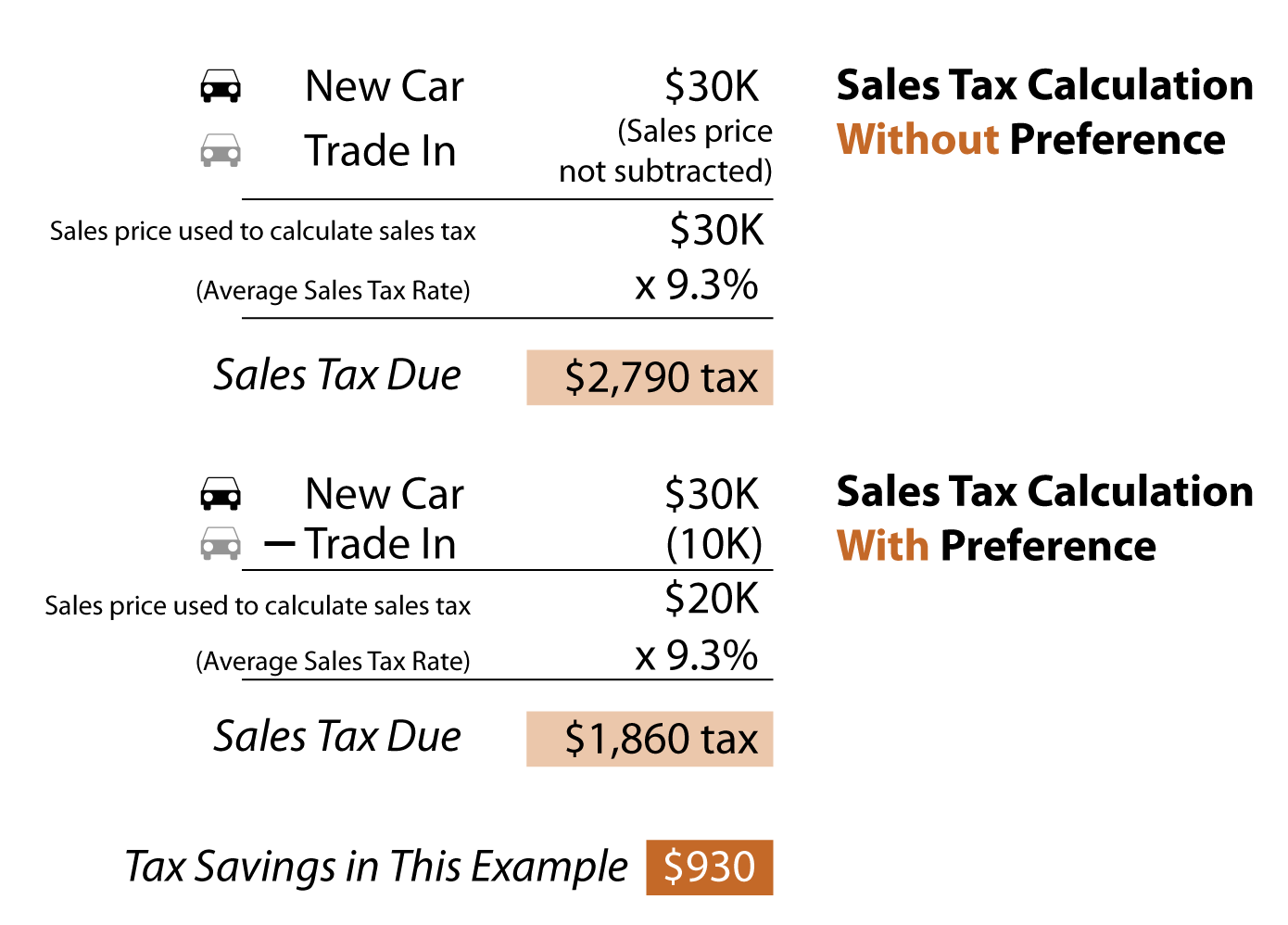
A person pays less in sales or use tax when purchasing an item (for example, a vehicle, airplane, or a boat) if the person trades in an item of “like-kind” to the seller at the time of the purchase. The reduction in sales or use tax is accomplished by “excluding” (subtracting) the value of the trade-in item when determining the price that is used to calculate sales or use tax.
The preference applies only to transactions involving goods, not services, and is limited to situations where:
- The buyer delivers the trade-in property to the seller at the time of sale (no future delivery);
- The trade-in property is considered as part of the payment for the purchase; and
- The trade-in property is “of a like-kind," meaning a vehicle for a vehicle (pick-up traded in on sedan purchase), or an appliance for an appliance (electric stove traded in on a gas range).
Pre-1984
People with a “like kind” good to trade in towards the purchase of an item paid the same in sales or use tax as purchasers without a trade-in.
November 1984
Washington voters passed Initiative No. 464 (I-464), which allowed the value of trade-ins of like-kind items to be excluded when calculating the sales tax due on a purchase of goods. I-464 was strongly supported by Washington auto dealers. Other proponents included consumer groups, farm equipment dealers, and boat manufacturers and dealers. I-464 took effect December 6, 1984.
The Department of Revenue (DOR) filed a proposed emergency rule immediately after the initiative passed, clarifying the changes for businesses and consumers. The initiative language did not include a specific trade-in provision for use tax, but DOR interpreted the exclusion to also apply to use tax transactions.
The tax preference has not been substantively altered since it was enacted.
2004
As part of the bill related to the Streamlined Sales and Use Tax Agreement, the Legislature clarified that eligible trade-in property must be “separately stated” in the calculation that determines the selling price.
Motor Vehicle Tax Also Calculated On Selling Price
In addition to reducing sales and use taxes, this preference also reduces collections of motor vehicle (MV) sales tax. Since 2003, people who buy or lease a motor vehicle in Washington pay a MV sales tax of 0.3 percent. Like sales and use taxes, the MV tax is calculated on the selling price of a motor vehicle. This preference reduces that selling price by subtracting the value of the trade-in.
Revenue from the MV sales tax is deposited into the multimodal transportation account which is used for grants to aid local governments in funding projects such as park and ride lots, transit services, and capital projects to improve transportation system connectivity and efficiency.
Vehicle Sales Involving Trade-ins
Auto industry publications indicate that, for U.S. vehicle sales in 2014:
- 48% of new vehicle sales involved trade-ins
- 29% of used vehicle sales involved trade-ins
What are the public policy objectives that provide a justification for the tax preference? Is there any documentation on the purpose or intent of the tax preference?
This preference was enacted via Washington’s initiative process rather than legislative action. Its adoption in 1984 preceded the 2013 legislative requirement to include a tax preference performance statement.
Reduce the Amount on Which Sales Tax Is Paid
The initiative language adopted by Washington voters specifically stated the purpose was “to reduce the amount on which sales tax is paid by excluding the trade-in value of certain property from the amount that is taxable.” The issue was described as an inequity that could be remedied by calculating the sales tax on the “net” price (initial sale price less trade-in value).
Additional Inferred Objectives
JLARC staff infer two additional objectives of the preference based on declarations included directly in the “Statement for” section of the voters’ pamphlet as, as well as newspaper articles and editorials.
- Make Washington consistent with other states that allowed a trade-in credit; and
- “Stimulate sales” and “offset any possible loss of revenue” caused by the preference (directly quoting phrases in the “Statements for” section of the voters’ pamphlet supporting I-464).
What evidence exists to show that the tax preference has contributed to the achievement of any of these public policy objectives?
Reduce the Amount on Which Sales Tax Is Paid
The preference is achieving the stated, voter-approved public policy objective of reducing the amount of sales tax paid on purchases when property is traded in. It functions to reduce the “selling price” of such purchases, upon which the sales or use tax is calculated.
Make Washington Consistent with Other States
The preference achieves the additional inferred objective of making Washington’s tax treatment for trade-in property consistent with many other states that impose sales tax. Forty-one states provide a sales tax exemption on trade-ins, with eleven of these states providing some limits on the amount or type of trade-in. (See the “Other States with Similar Tax Preference?” tab).
Stimulate Sales and Offset Loss of Revenue
While the preference may have stimulated additional sales, JLARC staff estimate the tax revenue generated from these sales does not offset the revenue lost due to the preference.
The analysis presented here focuses on vehicle sales because 82 percent of reported trade-in value in Fiscal Year 2015 was from new and used vehicle transactions. JLARC staff did not estimate results for other types of trade-ins, but their relatively smaller size would not impact the overall conclusion.
To assess the likelihood that the preference stimulated sales and generated enough tax revenue to offset any revenue losses due to the preference, JLARC staff incorporated two factors:
- Buyer responsiveness to vehicle price changes – The preference can be viewed as a reduction in vehicle price. JLARC staff calculated estimated values of statewide increased vehicle sales using a range of estimates of how responsive potential vehicle buyers are to vehicle price changes.
Based on a review of economic research literature on vehicle sales, JLARC staff identified a range of possible price response rates. These rates are what economists refer to as “price elasticities of demand.”
The elasticities range from a low of negative 0.2 to a high of negative 2.0. At an elasticity of negative 2.0, a 1 percent reduction in vehicle prices would result in a 2 percent increase in demand for vehicles. This analysis measures the change in demand for vehicles as the change in the dollar amount of sales. - Statewide revenue increases from additional vehicle sales – JLARC staff used the REMI model to estimate tax revenue gains from increased consumer expenditures on vehicle purchases involving a trade-in. The REMI model is a macroeconomic impact model of the state’s economy that accounts for changes in consumer expenditures, other indirect economic activities as a result of consumer expenditures, and total tax revenues from all activities. Use of the REMI model offers a comprehensive look at revenue gains beyond additional taxes on motor vehicles. JLARC staff used the model to estimate a tax revenue change for the elasticities in the range described above.
See Technical Appendix tab 1 for more information about the REMI model and Technical Appendix tab 2 for a step-by-step illustration of the calculations.
Below is a series of questions and answers based on the range of elasticities used in the analysis. These estimates are for Fiscal Year 2016. For all elasticities in the range, the amount of sales tax revenue lost due to the preference exceeds the estimated amount of all tax revenue gained from increased sales. This same result held in other fiscal years we modeled.
|
Questions
answered to reach the conclusion |
If elasticity is -0.2 |
If elasticity is -2.0 |
|
How
much did the preference reduce the price of a vehicle? |
3.6% |
3.6% |
|
Based on Department of Revenue and auto industry data
concerning auto sales and trade-ins, a buyer saved an average of 3.6% on the
price of a vehicle purchase involving a trade-in due to the reduction in
sales tax. |
||
|
How
much did this price reduction stimulate vehicle sales? |
$26.4 million |
$263.8 million |
|
The estimate of additional sales for FY 2016 varies based
on a range of assumptions of how responsive potential vehicle buyers are to a
reduction in vehicle price. |
||
|
How
much tax revenue was generated from these additional sales? |
$3.1 million |
$31.3 million |
|
The estimate of how much additional tax revenue would be generated
in FY 2016 is based on the results of the REMI model and the estimates of
additional vehicle sales in the row above. It includes taxes on vehicle sales directly as well as taxes from the other indirect activities in the economy that occur when consumers increase spending. |
||
|
How
much sales tax revenue was lost due to the preference? |
$182 million |
$182 million |
|
The amount is based on an average for fiscal years 2013-2015
for vehicle transactions involving trade-ins, adjusted to FY 2016. The amount does not include trade-ins for
other goods like airplanes, boats, farm machinery, or appliances. |
||
|
Does
the additional tax revenue generated offset the sales tax revenue lost? |
No. Net loss of $178.9
million |
No. Net loss of $150.7
million |
|
Estimates of the sales tax revenue lost
exceed estimates of tax revenue gains. Even
with the most optimistic elasticity assumption (-2.0), sales tax revenue lost
is $150.7 million more than the tax revenue gained from additional sales.
|
Other factors driving vehicle purchasing decisions
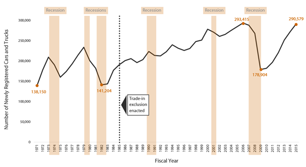
Information from additional sources suggests that other factors may be bigger drivers of vehicle purchasing decisions than an average 3.6 percent reduction in price. For example, the number of newly registered vehicles (vehicles that have not previously been titled) in Washington varies with more general economic conditions.
To what extent will continuation of the tax preference contribute to these public policy objectives?
Continuing the tax preference will continue to reduce the amount on which sales tax is paid for purchases involving trade-ins and make Washington’s taxation consistent with many other states. While the preference may continue to stimulate some additional sales, it is unlikely to generate additional sales tax revenue to make up the difference in the tax loss due to the preference.
Who are the entities whose state tax liabilities are directly affected by the tax preference?
Direct Beneficiaries
The direct beneficiaries of this preference are people and businesses that purchase goods and trade in like-kind goods at the time of sale. Specific data is not available to determine the number of beneficiaries. For Fiscal Year 2015, new and used vehicles made up the majority (82 percent) of the value of like-kind goods traded in. Other purchases involving trade-ins included recreational vehicles, industrial and farm machinery and equipment, auto parts and tires, boats, motorcycles, and all-terrain vehicles.
Indirect Beneficiaries
New and used automobile dealers are the largest indirect beneficiaries of the preference. The preference may encourage people considering the purchase of a new or used vehicle to do so through a dealership. The trade-in sales tax exclusion is only available if the buyer presents a like-kind item to trade in at the time of sale. People selling their existing vehicles independently do not generally benefit from the preference.
New and used motor vehicle dealers must obtain a license with the Department of Licensing (DOL). As of April 2016, DOL reports there were 400 new motor vehicle dealers and 1,498 used motor vehicle dealers licensed in Washington. JLARC staff identified 838 new and used vehicle sale businesses reporting trade-ins in Fiscal Year 2015.
What are the past and future tax revenue and economic impacts of the tax preference to the taxpayer and to the government if it is continued?
JLARC staff estimate direct beneficiaries of the trade-in preference saved $239.1 million in Fiscal Year 2015 and will save $591.4 million for the 2017-19 Biennium due to this preference. JLARC staff used Department of Revenue tax return data and Department of Licensing registration data to estimate the beneficiary savings, which are comprised of three components:
- State sales and use tax (6.5 percent)
- Local sales and use tax (about 2.5 percent)
- Additional motor vehicle sales tax (0.3 percent)
| Fiscal Year | State Sales/Use Tax | Local Sales/Use Tax | 0.3% Motor Vehicle Tax | Total Beneficiary Savings |
|---|---|---|---|---|
| 2014 | $161,765,000 | $61,058,000 | $5,957,000 | $228,780,000 |
| 2015 | $168,787,000 | $64,129,000 | $6,221,000 | $239,137,000 |
| 2016 | $176,008,000 | $67,668,000 | $6,488,000 | $250,164,000 |
| 2017 | $194,308,000 | $74,704,000 | $7,162,000 | $276,174,000 |
| 2018 | $204,882,000 | $78,769,000 | $7,552,000 | $291,204,000 |
| 2019 | $211,243,000 | $81,215,000 | $7,786,000 | $300,244,000 |
| 2017-19 Biennium | $416,125,000 | $159,984,000 | $15,338,000 | $591,448,000 |
If the tax preference were to be terminated, what would be the negative effects on the taxpayers who currently benefit from the tax preference and the extent to which the resulting higher taxes would have an effect on employment and the economy?
If the tax preference were terminated, individuals and businesses would pay more sales or use tax on purchases of goods where they trade in like-kind goods. Also, people and businesses would pay more motor vehicle sales tax on purchases of vehicles where they trade in a used vehicle
Vehicle dealers likely may see a reduction in sales from an increase in sales price, which could result in a decrease in the number of or amount spent on consumer vehicle purchases.
However, JLARC staff’s analysis indicates termination of the preference would likely result in an overall increase in tax revenue. The reduction in tax revenue from fewer vehicle sales would be more than offset by the additional sales tax collected by removing the trade-in tax preference.
Do other states have a similar tax preference and what potential public policy benefits might be gained by incorporating a corresponding provision in Washington?
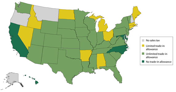
Of the 45 states and the District of Columbia that impose sales and use taxes, five do not provide any form of sales tax reduction for trade-ins: California, District of Columbia, Hawaii, Maryland, and North Carolina.
Thirty states, including Washington, provide a largely unrestricted sales tax exemption for trade-in property. Like Washington, most states that allow a trade-in exemption clarify it is for “like kind” property.
Eleven states provide a trade-in exclusion that is limited in some manner. Most of these are for motor vehicles. Some states also allow a trade-in exclusion for watercraft, vessels, or farm machinery. Ohio provides a trade-in exclusion for new (but not used) vehicle or watercraft purchases.
REMI Overview
JLARC staff used Regional Economic Models, Inc.’s (REMI) Tax-PI software (v 1.7.105) to model the economic impacts for three tax preference reviews in the 2016 report: trade-ins, timber, and data centers.
REMI software is used by 34 state governments and dozens of private sector consulting firms, research universities, and international clients.
Model Is Tailored to Washington and Includes Government Sector
Tax-PI is an economic impact tool for evaluating the fiscal and economic effects and the demographic impacts of tax policy change. The software includes various features that make it particularly useful for analyzing the economic and fiscal impacts of tax preferences:
- REMI staff consulted with staff from the Office of Financial Management (OFM) and customized a statewide model to reflect Washington’s economy;
- The model contains 160 industry sectors, based on the North American Industry Classification System (NAICS) codes;
- In contrast to other modeling software, Tax-PI includes state and local government as a sector. This permits users to see the trade-offs associated with tax policy changes (e.g., effects on the state’s economy from both increased expenditures by businesses due to a tax preference along with decreased spending by government due to the revenue loss);
- For current revenue and expenditure data, users can input information to reflect their state’s economic and fiscal situation. This allows JLARC staff to calibrate a state budget using up-to-date information from the Economic and Revenue Forecast Council (ERFC) and the Legislative Evaluation and Accountability Program (LEAP); and
- The model can forecast economic and revenue impacts multiple years into the future.
Results the Model Provides
The REMI model accounts for the direct, indirect, and induced effects as they spread through the state’s economy, which allows users to simulate the full impact of tax policy change over time.
- Direct effects are industry specific and capture how a target industry responds to a particular policy change (e.g., changes in industry employment following a change in tax policy);
- Indirect effects capture employment and spending decisions by businesses in the targeted industry’s supply chain that provide goods and services; and
- Induced effects capture the in-state spending and consumption habits of employees in targeted and related industries.
The REMI model produces year-by-year estimates of the total statewide effects of a tax policy change. Impacts are measured as the difference between a baseline economic and revenue forecast and the estimated economic and revenue effects after the policy change.
What the Model Includes
The REMI model is a macroeconomic impact model that incorporates aspects of four major economic modeling approaches: input-output, general equilibrium, econometric, and new economic geography. The foundation of the model, the inter-industry matrices found in the input-output models, captures Washington’s industry structure and the transactions between industries. Layered on top of this structure is a complex set of mathematical equations used to estimate how private industry, consumers, and state and local governments respond to a policy change over time.
- The supply side of the model includes many economic variables representing labor supply, consumer prices, and capital and energy costs with elasticities for both the consumer and business sectors.
- Regional competitiveness is modeled via imports, exports, and output.
- Demographics are modeled using population dynamics (births, deaths, and economic and retirement migration) and includes cohorts for age, sex, race, and retirement.
- Demographic information informs the model’s estimates for economic consumption and labor supply.
- The dynamic aspect comes from the ability to adjust variables over time as forecasted economic conditions change.
While the model is complex and forecasting involves some degree of uncertainty, Tax-PI provides a tool for practitioners to simulate how tax policy and the resulting industry changes affect Washington’s economy, population, and fiscal situation.
Three Approaches Support Conclusions about Revenue Loss
One inferred objective of the tax preference for trade-ins is to stimulate sales and offset any possible loss of revenue caused by the preference. The conclusion of this review: While the preference may have stimulated additional sales, JLARC staff estimate the tax revenue generated from these sales does not offset the revenue lost due to the preference.
This technical appendix provides more detail on the approaches and calculations JLARC staff used to reach that conclusion. The analyses focused on vehicle sales because 82 percent of reported trade-in value in Fiscal Year 2015 was from new and used vehicle transactions. JLARC staff evaluated net revenue impacts using three approaches:
- REMI Model – Single Elasticity in the Model
This approach mirrors REMI analyses JLARC staff have conducted on other tax preferences. It considers both the tax revenue gained from a reduction in consumer prices due to the preference and the tax revenue lost due to the preference and decreased government spending. In terms of how consumers respond to a change in vehicle prices, this approach used the value internal to the REMI model. - Sales Tax Revenue Changes – Range of Elasticities
In this approach, JLARC staff estimated sales tax revenue changes due to changes in vehicle sales and considered a range of estimates of how responsive potential vehicle buyers are to vehicle price changes. The degree of responsiveness – the “price elasticity of demand” – ranged from a low of negative 0.2 to a high of negative 2.0. - REMI Model – All Tax Revenue – Range of Elasticities
This approach combined both the REMI model and the range of elasticities reflecting consumer responsiveness to vehicle price changes. The approach considers all tax revenues, not just sales tax. The results presented in the “Are Objectives Being Met?” tab come from this combined approach.
The results from all three approaches support the conclusion that tax revenue generated by any additional vehicle sales does not offset the revenue lost due to the preference.
Approach #1 – REMI Model – Single Elasticity in the Model
User Inputs in REMI
REMI’s Tax-PI model allows users to model policy changes and analyze the estimated impacts to the Washington economy, both in terms of economic activity and government finances. (See Technical Appendix 1 for an overview of the REMI model.)
Prior to running modeling scenarios, users must make a series of choices about how to set up the modeling environment by building a state budget and calibrating the model accordingly. JLARC staff used the November 2015 revenue estimates produced by the Economic and Revenue Forecast Council (ERFC) and budgeted expenditures for FY 2014 and 2015, as reported by the Legislative Evaluation and Accountability Program (LEAP) Committee. This data represents the budget and revenue data in the model and serves as the “jump off” point for Tax-PI’s economic and fiscal estimates. Because Tax-PI is a forecasting tool, JLARC staff was unable to model the economic impact of the tax preference beginning in 2006.
In addition to establishing a budget and inputting expected revenue values, users must specify whether government expenditures are determined by demand or revenue. “By demand” imposes a level of government spending in future years that is necessary to maintain the same level-of-service as the final year in which budget data is entered whereas “by revenue” ties government expenditures to estimated changes in revenue collections.
Users may also elect to impose a balanced budget restriction or leave the model unconstrained. The balanced budget feedback forces revenue and expenditures to be equivalent and thus may impose some limitations on economic activity.
By setting expenditures to be determined by demand, users avoid making assumptions about how policymakers may alter spending priorities in the future. In addition, users essentially establish the current budget allocation as carry-forward levels for each expenditure category.
JLARC staff ran the reported scenario with expenditures set to be determined by demand and with the balanced budget feedback option turned on.
Data for the REMI Model
The REMI model comes with historical economic and demographic data back to 1990. The data comes from federal government agencies such as the U.S. Census Bureau, U.S. Energy Information Administration, the Bureau of Labor Statistics, and the Bureau of Economic Analysis. As described above, current revenue and expenditure data for Washington comes from ERFC and LEAP, respectively. The data used to build the modeling scenario described in section three is from JLARC staff estimated beneficiary savings based on Department of Revenue (DOR) tax records.
Modeling the Scenario
JLARC staff used REMI to evaluate the economic and revenue response to a change in the price of new and used vehicles. Specifically, JLARC staff modeled a scenario simulating the lowering of vehicle prices for consumers and decreasing government spending by the amount of the estimated beneficiary savings. The analysis compared the effects of increased tax revenue associated with increased consumer spending with the foregone tax revenue resulting from the preference and reduced government spending.
In this approach, JLARC staff changed the following policy variables in REMI:
- Decreased “Government Spending” by the estimated amount of beneficiary savings attributable to vehicle sales, calculated using DOR data showing the amount of trade-in deductions reported.
- Decreased the consumer price for the policy variables “New Motor Vehicles” and “Net Purchases of Used Motor Vehicles.”
Table 1 shows the REMI results for the changes to these three policy variables for Fiscal Years 2015-2020. The price change affected consumers’ purchasing power for vehicles, and includes the substitution effect that simulates consumers changing demand for one good based on a change of price of another good. The reduction in the price of automobiles increased purchases of autos while decreasing purchases of other goods. In contrast, government spending declined.
| Table 1 - Policy Variable Changes (in Millions of Dollars) |
||||||
|---|---|---|---|---|---|---|
| Fiscal Year | 2015 | 2016 | 2017 | 2018 | 2019 | 2020 |
| Consumer Price - New Motor Vehicles | -$125.1 | -$126.6 | -$129.2 | -$131.1 | -$133.4 | -$136.7 |
| Consumer Price - Net Purchases of Used Motor Vehicles | -$49.9 | -$55.4 | -$62.0 | -$67.4 | -$71.9 | -$75.3 |
| Government Spending | -$175.0 | -$182.0 | -$191.2 | -$198.5 | -$205.3 | -$212.0 |
REMI then allows a user to calculate the net revenue changes associated with the effects shown in Table 1. Table 2 shows the estimated net revenue effect of the trade-in deduction for Fiscal Years 2015-2020. The REMI analysis includes the net revenue effect of lower consumer prices and lower government spending, while the beneficiary savings represents the foregone revenue due to the tax preference.
Although the vehicle price reduction did result in an increase in vehicle sales, and therefore an increase in sales tax revenue, the gain was more than offset by the loss of sales tax revenue due to the preference and the reduction in government spending.
| Table 2 - Net Revenue Effect (in Millions of Dollars) | ||||||
|---|---|---|---|---|---|---|
| Fiscal Year | 2015 | 2016 | 2017 | 2018 | 2019 | 2020 |
| Revenue Change - REMI Analysis | $12.2 | $25.6 | $27.6 | $29.0 | $30.2 | $31.4 |
| Revenue Decrease - Beneficiary Savings | -$175.0 | -$182.0 | -$191.2 | -$198.5 | -$205.3 | -$212.0 |
| Net Revenue Effect | -$162.8 | -$156.4 | -$163.6 | -$169.5 | -$175.1 | -$180.6 |
A limitation of this approach, however, is that REMI users are not able to change the price elasticity of demand for vehicles. Instead, this is a fixed value in the REMI model of approximately -1.65. As such, modeling the price change of new and used vehicles in REMI would use that elasticity. In order to evaluate the effects of the tax preference using various assumptions for the price elasticity of demand for vehicles, JLARC staff developed two different approaches, both of which used the concept of price elasticity of demand.
Approach #2 – Sales Tax Revenue Changes – Range of Elasticities
Approach #2 focuses on sales tax revenues and introduces the concept of consumer responsiveness to changes in vehicle prices.
What is Price Elasticity of Demand?
To approximate a potential response of vehicle sales to a tax preference that effectively reduces vehicle prices, JLARC staff used price elasticity of demand, the measure of responsiveness of the quantity demanded of a good or service to a change in its price. Specifically, the values of elasticities in this report refer to the percentage change in quantity demanded in response to a one percent change in price.
Price elasticities with an absolute value less than 1 are considered inelastic (purchases deemed essential and/or without adequate substitutions available) whereas absolute values greater than 1 are elastic (purchases may be delayed or substitutions are available). A value of 1 indicates unit elasticity or an equivalent percent change in quantity purchased relative to the percent change in price. The price elasticities of demand included in this analysis are negative, indicating a decrease in price would result in an increase in demand.
Price Elasticity of Demand for Automobiles
The price elasticity of demand for vehicle purchases is not a definitively established amount, as there are many variables that potentially impact consumer behavior. For example, the elasticities associated with vehicle sales vary due to factors such as geography (urban vs. rural), make and model of automobile, and year (new vs. used). JLARC staff reviewed literature and found that various studies have arrived at a wide range of price elasticities of demand, and this analysis therefore presents a range of elasticities informed by that review.
JLARC staff approximated the effect that a price change resulting from a reduction in sales tax could have on demand for vehicles. Rather than assigning one elasticity for the estimate, JLARC staff calculated potential changes in demand and, consequently, vehicle purchases, based on the range of elasticities found in the literature. The range of elasticities used in this analysis is -0.2, -0.5, -0.8, -1.0, -1.2, -1.5, -1.8, -2.0. See the list of references at the end of this appendix for the literature JLARC staff reviewed in developing this range.
Evaluating Change in Vehicle Price and Demand
Because the price elasticities of demand described above indicate responsiveness to changes in price, the next portion of the analysis required estimation of the percentage change in the price of vehicles that involved a trade-in that can be attributed to the trade-in deduction. This percentage change in vehicle prices is multiplied by the range of elasticities to estimate the percentage change in vehicle demand. This change, in turn, is multiplied by a base amount of taxable sales and to estimate the additional vehicle sales stimulated by the change in price.
To estimate the percentage change in price, JLARC staff used Fiscal Year 2013-2015 data reported to the Department of Revenue (DOR) by automobile dealerships for taxable sales and for reported deductions pursuant to the trade-ins tax preference.
- The calculation begins with taxable sales reported by automobile dealerships to DOR.
- The taxable sales amount includes parts and service sales, which is not part of the analysis. According to data from the National Automobile Association of America parts and service sales are 11.4 percent of total dealership sales.
- Reducing taxable sales by 11.4 percent generates estimated taxable vehicle sales.
- The deduction reported to DOR by automobile dealerships represents amounts deducted as they are not taxable pursuant to the trade-in deduction.
- Adding taxable vehicle sales to the amount of the deduction results in estimated total vehicle sales.
- Taxable vehicle sales is multiplied by 41.4 percent to estimate total trade-in sales.
To estimate the share of sales that involve a trade-in, JLARC staff relied on data from the National Automobile Association of America showing the share of vehicle sales that are new or used, and data from Edmunds.com concerning the percentage of new and used vehicle sales that involve a trade-in. Table 3 shows how these percentages are multiplied together for each category of sale, then added together to estimate at 41.4 percent the trade-in share of total vehicle sales.
| Table 3 - Estimating Trade-in Share of Total Vehicle Sales | |||
|---|---|---|---|
| Category | % of Sales | Trade-In Share | Total Share |
| New | 65.0% | 48% | 31.2% |
| Used | 35.0% | 29% | 10.1% |
| Trade-In Share of Total Auto Sales 41.4% | |||
- To estimate the tax that would be due on vehicle sales absent the tax preference, total trade-in sales is multiplied by an estimated tax rate. The tax rate comprises three components, shown in table 4.
| Table 4 - Sales Tax Rates | |||
|---|---|---|---|
| State | Local | MV Tax | Total |
| 6.5% | 2.48% | 0.3% | 9.28% |
- Total trade-in vehicle cost is estimated by adding total trade-in sales to total trade-in sales tax. The steps used to arrive at this total are shown in table 5.
| Table 5 - Estimating Base Vehicle Spending | ||||||||
|---|---|---|---|---|---|---|---|---|
1 |
2 |
3 |
4 |
5 |
6 |
7 |
8
|
|
Fiscal Year |
Taxable Sales |
Parts/ Service Adj. |
Taxable Vehicle Sales |
Deduction |
Total Vehicle Sales |
Total Trade-in Sales |
Total Trade-in Sales Tax |
Total Trade-in Vehicle Cost |
| 2013 | $9,050,005,038 | -11.4% | $8,018,304,464 | $1,816,820,555 | $9,835,125,019 | $4,067,035,106 | $377,420,858 | $4,444,455,964 |
| 2014 | $9,909,834,610 | -11.4% | $8,780,113,464 | $1,887,511,267 | $10,667,624,731 | $4,411,291,590 | $409,367,860 | $4,820,659,450 |
| 2015 | $10,802,529,048 | -11.4% | $9,571,040,737 | $1,955,421,731 | $11,526,462,468 | $4,766,439,412 | $442,325,577 | $5,208,764,989 |
| Average | $9,920,789,565 | -11.4% | $8,789,819,555 | $1,886,584,518 | $10,676,404,073 | $4,414,922,036 | $409,704,765 | $4,824,626,801 |
- Estimating the price change percentage that the sales tax difference represents begins with the deduction reported to DOR by automobile dealerships.
- This deduction is multiplied by the estimated tax rate to estimate the sales tax difference. This number is the numerator used to calculate the price change percentage.
- Total trade-in vehicle cost is the denominator used to calculate the price change percentage.
- The number from step 10 is divided by the number from step 11 to estimate the price change percentage. The steps used to estimate this percentage are shown in table 6.
| Table 6 - Estimating Price Change due to Deduction | ||||
|---|---|---|---|---|
9 |
10 |
11 |
12 |
|
Fiscal Year |
Deduction |
Sales Tax Difference |
Total Trade-in Vehicle
Cost |
Price Change % |
| 2013 | $1,816,820,555 | -$168,600,948 | $4,444,455,964 | -3.79% |
| 2014 | $1,887,511,267 | -$175,161,046 | $4,820,659,450 | -3.63% |
| 2015 | $1,955,421,731 | -$181,463,137 | $5,208,764,989 | -3.48% |
| Average | $1,886,584,518 | -$175,075,043 | $4,824,626,801 | -3.63% |
JLARC staff multiplied the price change percentage with the various price elasticities to estimate a range of percent demand changes, which are shown in table 7.
| Table 7 - Estimated Percent Demand Changes | ||||||||||
|---|---|---|---|---|---|---|---|---|---|---|
Fiscal Year |
Price Change % |
-0.20 |
-0.50 |
-0.80 |
-1.00 |
-1.20 |
-1.50 |
-1.65 |
-1.80 |
-2.00 |
| 2013 | -3.79% | 0.76% | 1.90% | 3.03% | 3.79% | 4.55% | 5.69% | 6.26% | 6.83% | 7.59% |
| 2014 | -3.63% | 0.73% | 1.82% | 2.91% | 3.63% | 4.36% | 5.45% | 6.00% | 6.54% | 7.27% |
| 2015 | -3.48% | 0.70% | 1.74% | 2.79% | 3.48% | 4.18% | 5.23% | 5.75% | 6.27% | 6.97% |
| Average | -3.63% | 0.73% | 1.81% | 2.90% | 3.63% | 4.35% | 5.44% | 5.99% | 6.53% | 7.26% |
These percentages were multiplied with base taxable sales to estimate a range of marginal taxable sales, shown in table 8.
| Table 8 - Estimated Marginal Taxable Sales(in Millions of Dollars) | ||||||||||
|---|---|---|---|---|---|---|---|---|---|---|
Fiscal Year |
Base Taxable Sales |
-0.20 |
-0.50 |
-0.80 |
-1.00 |
-1.20 |
-1.50 |
-1.65 |
-1.80 |
-2.00 |
| 2013 | $3,315.7 | $25.2 | $62.9 | $100.6 | $125.8 | $150.9 | $188.7 | $207.5 | $226.4 | $251.6 |
| 2014 | $3,630.8 | $26.4 | $66.0 | $105.5 | $131.9 | $158.3 | $197.9 | $217.7 | $237.5 | $263.9 |
| 2015 | $3,957.8 | $27.6 | $68.9 | $110.3 | $137.9 | $165.5 | $206.8 | $227.5 | $248.2 | $275.8 |
| Average | $3,634.8 | $26.4 | $65.9 | $105.5 | $131.9 | $158.2 | $197.8 | $217.6 | $237.4 | $263.7 |
Comparing Marginal Sales Tax Revenue to Revenue Lost Due to Preference
The exercise above led to an estimate of the increase in vehicle sales associated with each of the elasticities in the range.
The last step was to calculate the sales tax revenue gains for each of the increases in vehicle sales, then compare these to the sales tax revenue that is foregone due to the trade-in preference.
JLARC staff averaged the marginal sales estimated for Fiscal Years 2013, 2014, and 2015 for each value of elasticity above. Multiplying these values by a tax rate of 9.28 percent (Table 4) yields estimated marginal sales tax revenues.
The tax rate comprises the 6.5 percent state rate, an estimated average local sales tax rate of 2.48 percent, and a 0.3 percent motor vehicle tax pursuant to RCW 82.08.020(3) that is deposited in the multimodal transportation account.
The marginal revenue amounts are compared with the offsetting revenue cost of the preference, averaged for FY13-FY15, with a growth rate applied for FY16. The growth rate reflects growth in personal consumption expenditures for new and used vehicles in REMI’s baseline forecast.
The results of this analysis are shown in Table 9. For every elasticity in the range, the sales tax revenue lost exceeds any sales tax revenue gains.
| Table 9 - Estimated Marginal Sales Tax Revenue - Tax Rate - FY16 (in Millions of Dollars) | ||||||||||
|---|---|---|---|---|---|---|---|---|---|---|
Fiscal Year |
Tax Rate |
-0.20 |
-0.50 |
-0.80 |
-1.00 |
-1.20 |
-1.50 |
-1.65 |
-1.80 |
-2.00 |
| 2013 | 9.28% | $2.33 | $5.84 | $9.34 | $11.67 | $14.01 | $17.51 | $19.26 | $21.01 | $23.35 |
| 2014 | 9.28% | $2.45 | $6.12 | $9.79 | $12.24 | $14.69 | $18.36 | $20.20 | $22.04 | $24.49 |
| 2015 | 9.28% | $2.56 | $6.40 | $10.24 | $12.80 | $15.35 | $19.19 | $21.11 | $23.03 | $25.59 |
| Average | 9.28% | $2.45 | $6.12 | $9.79 | $12.24 | $14.68 | $18.36 | $20.19 | $22.03 | $24.47 |
| Estd. Beneficiary Savings | -$182.0 | -$182.0 | -$182.0 | -$182.0 | -$182.0 | -$182.0 | -$182.0 | -$182.0 | -$182.0 | |
| Net Revenue | -$179.6 | -$175.9 | -$172.2 | -$169.8 | -$167.3 | -$163.6 | -$161.8 | -$160.0 | -$157.5 | |
Approach #3 -- REMI Model – All Tax Revenue – Range of Elasticities
Approach #3 combines the range of elasticities from Approach #2 with use of the REMI model. Approach #2 is limited because it only captures potential marginal revenue attributable to the sales tax on vehicles, and not dynamic revenue impacts from other taxes or other economic activity supported by the additional vehicle purchases. JLARC staff used REMI to estimate this dynamic impact of the marginal auto sales. As in Approach #2, the marginal revenue amounts are compared with the offsetting revenue cost of the preference, averaged for FY13-FY15, with a growth rate applied for FY16. The results of this approach are summarized in the “Are Objectives Being Met?” tab, and they are shown in Table 10. For every elasticity in the range, the sales tax revenue lost exceeds any tax revenue gains.
| Table 10
- Estimated REMI Results of Elasticity Analysis (in Millions of Dollars) |
|||||||||
|---|---|---|---|---|---|---|---|---|---|
| Elasticity | -0.20 | -0.50 | -0.80 | -1.00 | -1.20 | -1.50 | -1.65 | -1.80 | -2.00 |
| % Change in Price | -3.6% | -3.6% | -3.6% | -3.6% | -3.6% | -3.6% | -3.6% | -3.6% | -3.6% |
| % Change in Demand | 0.7% | 1.8% | 2.9% | 3.6% | 4.4% | 5.4% | 6.0% | 6.5% | 7.3% |
| Base Taxable Sales | $3,634.8 | $3,634.8 | $3,634.8 | $3,634.8 | $3,634.8 | $3,634.8 | $3,634.8 | $3,634.8 | $3,634.8 |
| Additional Sales from Increased Demand | $26.4 | $65.9 | $105.5 | $131.9 | $158.3 | $197.8 | $217.6 | $237.4 | $263.8 |
| Revenue from Additional Sales | $3.1 | $7.8 | $12.5 | $15.6 | $18.8 | $23.4 | $25.7 | $28.1 | $31.3 |
| Estimated Forgone Revenue | -$182.0 | -$182.0 | -$182.0 | -$182.0 | -$182.0 | -$182.0 | -$182.0 | -$182.0 | -$182.0 |
| Net Revenue | -$178.9 | -$174.2 | -$169.5 | -$166.4 | -$163.2 | -$158.6 | -$156.3 | -$153.9 | -$150.7 |
To build this simulation, JLARC staff amended the policy variable for personal consumption expenditures by the amount of marginal sales calculated for each elasticity value.
- The model includes policy variables for two types of automobile purchases, New Motor Vehicles and Net Purchases of Used Motor Vehicles. The marginal sales amount was distributed in proportion to REMI’s baseline personal consumption expenditures for these two variables.
- Because the personal consumption expenditures for these variables grow in the REMI’s baseline forecast, JLARC staff grew the marginal sales amounts by the same growth rates in out years.
- Revenue changes reflect only the increase in personal consumption expenditures, and do not show substitution effects on other consumption categories that would be expected if the change in automobile consumption were driven by a change in vehicle price.
- Revenue changes also do not reflect changes in revenue resulting from a reduction in government spending attributable to the revenue forgone due to the tax preference.
References
Dyckman, T. R..(1965). An Aggregate-Demand Model for Automobiles. Journal of Business, 38, 252-265. Retrieved from http://www.jstor.org/stable/2351061
Gwartney, J., and Richard Stroup. (1997). Economics: Private and Public Choice, 8th edition. New York, New York: Dryden.
Hymans, S. H.. (1970). Consumer Durable Spending: Explanation and Prediction. In Arthur N. Okun and George L. Perry (Eds.), Brookings Papers on Economic Activity (173-199). Washington, D.C.: The Brookings Institution. Retrieved from https://www.brookings.edu/wp-content/uploads/1970/06/1970b_bpea_hymans_ackley_juster.pdf
Juster, F. T., and Paul Wachtel. (1972). Anticipatory and Objective Models of Durable Goods Demand. American Economic Review, 62, 564-579. Retrieved from http://www.jstor.org/stable/1806099
Lave, C., and Kenneth Train. (Jan. 1979). A Disaggregate Model of Auto-Type Choice. Transportation Research, 13A, 1-9. Retrieved from https://www.researchgate.net/publication/256509538_A_Disaggregate_Model_of_Auto-Type_Choice
Levinsohn, J.. (1988). Empirics of Taxes on Differentiated Products: The Cast of Tariffs in the U.S. Automobile Industry. In Robert E. Baldwin (Ed.), Trade Policy Issues and Empirical Analysis (11-40). Chicago, Illinois: University of Chicago Press. Retrieved from http://www.nber.org/chapters/c5846.pdf
McCarthy, P. S.. (1996). Market Price and Income Elasticities of New Vehicle Demands. The Review of Economics and Statistics, 78, 543–547. http://doi.org/10.2307/2109802
Nerlove, M.. (1957). A Note on Long-Run Automobile Demand. Journal of Marketing, 22, 57-64. Retrieved from https://journals.sagepub.com/doi/pdf/10.1177/002224295702200109
Suits, D. B.. (1958). The Demand for New Automobiles in the United States 1929-1956. The Review of Economics and Statistics, 40, 273-280. http://doi.org/10.2307/1927419
Suits, D. B.. (1961). Exploring Alternative Formulations of Automobile Demand. The Review of Economics and Statistics, 43(1), 66-69. http://doi.org/10.2307/1926837
RCW 82.08.010
Definitions.
For the purposes of this chapter:
(1)(a)(i) "Selling price" includes "sales price." "Sales price" means the total amount of consideration, except separately stated trade-in property of like kind, including cash, credit, property, and services, for which tangible personal property, extended warranties, digital goods, digital codes, digital automated services, or other services or anything else defined as a "retail sale" under RCW 82.04.050 are sold, leased, or rented, valued in money, whether received in money or otherwise. No deduction from the total amount of consideration is allowed for the following: (A) The seller's cost of the property sold; (B) the cost of materials used, labor or service cost, interest, losses, all costs of transportation to the seller, all taxes imposed on the seller, and any other expense of the seller; (C) charges by the seller for any services necessary to complete the sale, other than delivery and installation charges; (D) delivery charges; and (E) installation charges.
[ 2014 c 140 § 11; 2010 c 106 § 210; 2009 c 535 § 303; 2007 c 6 § 1302; (2007 c 6 § 1301 expired July 1, 2008); 2006 c 301 § 2; 2005 c 514 § 110; 2004 c 153 § 406; 2003 c 168 § 101; 1985 c 38 § 3; 1985 c 2 § 2 (Initiative Measure No. 464, approved November 6, 1984); 1983 1st ex.s. c 55 § 1; 1967 ex.s. c 149 § 18; 1963 c 244 § 1; 1961 c 15 § 82.08.010. Prior: (i) 1945 c 249 § 4; 1943 c 156 § 6; 1941 c 178 § 8; 1939 c 225 § 7; 1935 c 180 § 17; Rem. Supp. 1945 § 8370-17. (ii) 1935 c 180 § 20; RRS § 8370-20.]
- Legislative Auditor Recommendation
- Letter from Commission Chair
- Commissioners’ Recommendation
- Agency Response
Legislative Auditor Recommendation
The Legislature should review and clarify the sales tax exemption for trade-ins because, while the preference is achieving the inferred objectives of reducing consumers’ taxes and making Washington’s tax treatment consistent with other states, it is not achieving the objective of stimulating enough additional sales to replace lost revenue.
Legislation Required: Yes.
Fiscal Impact: Depends on legislative action.

The Commission endorses the Legislative Auditor’s recommendation.
As the Legislature reviews this preference, the Commission notes that this tax preference is similar to the tax treatment of trade-ins in many other states, due to concerns of double taxation. Additionally, the JLARC staff’s review concludes the $182 million associated with automobile sales is estimated to only generate $31 million in new sales, causing a net loss of $151 million in tax revenue.
Joint Department of Revenue and Office of Financial Management Response